Understanding what RNN learns: Part 1
This tutorial will take you through a basic understanding of the working of RNN. You can have a lok at Chris Olah’s blog on RNN to understand RNN architecture.
This tutorial is a copy of a jupyter notebook, link to which is given at the bottom. The style used here is similar: grey section followed by ‘In’ is a python code and following grey section (after ‘Out’) is the corresponding output.
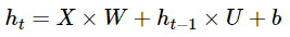
We will be using a simple RNN for which the cell-equation (not a standard name) is:

Setup:
Our aim in first problem is to predict the sum of 3 numbers with RNN. Thus for each input sequence [x0,x1,x2][x0,x1,x2], output should be

Note: I know the same can be achieved with a simple neural net, but to keep it simple we are setting the problem this way.
# Import modules
import numpy as np
from keras.models import Model
from keras.layers import Input, SimpleRNN# Data and model parameters
seq_len = 3   #Length of each sequence
rnn_size = 1  #Output shape of RNN
input_size = 10000 #Numbers of instances
Creating Data:
In :
all_feat = np.random.randint(low=0, high=10, size=(input_size,3,1))
all_feat[:5, :]
Out:
array([[[9],
        [0],
        [1]],       [[7],
        [6],
        [4]],       [[7],
        [8],
        [4]],       [[5],
        [5],
        [8]],       [[1],
        [7],
        [1]]])
In :
all_label = np.apply_along_axis(func1d=np.sum, axis=1, arr=all_feat)
all_label[:5]
Out:
array([[10],
       [17],
       [19],
       [18],
       [ 9]])
Define model
Our model will have only a Simple RNN.
Our expectation with RNN is that it will learn to pass the input as it is to next layer.
One more thing to note: to keep things simple to understand, we’ll use linear activation(y=f(x)=x)
x = Input(shape=(3,1,), name='Input_Layer')
y = SimpleRNN(rnn_size, activation='linear', name='RNN_Layer')(x)model = Model(inputs=x, outputs=y)model.summary()
Out:
________________________________________________________________
Layer (type)                 Output Shape              Param #
=================================================================
Input_Layer (InputLayer)     (None, 3, 1)              0
_________________________________________________________________
RNN_Layer (SimpleRNN)        (None, 1)                 3
=================================================================
Total params: 3.0
Trainable params: 3.0
Non-trainable params: 0.0
_________________________________________________________________
In:
model.compile(optimizer='adam', loss='mean_squared_error', metrics=['acc'])Time to train the model
In:
history = model.fit(x=all_feat, y=all_label, batch_size=4, epochs=5, validation_split=0.2, verbose=1)Out:
Train on 8000 samples, validate on 2000 samples
Epoch 1/5
8000/8000 [==============================] - 9s - loss: 52.2708 - acc: 0.1204 - val_loss: 2.8959 - val_acc: 0.2050
Epoch 2/5
8000/8000 [==============================] - 8s - loss: 2.3057 - acc: 0.2139 - val_loss: 1.5666 - val_acc: 0.2775
Epoch 3/5
8000/8000 [==============================] - 8s - loss: 0.9501 - acc: 0.3466 - val_loss: 0.4068 - val_acc: 0.5105
Epoch 4/5
8000/8000 [==============================] - 9s - loss: 0.1705 - acc: 0.7825 - val_loss: 0.0324 - val_acc: 1.0000
Epoch 5/5
8000/8000 [==============================] - 9s - loss: 0.0084 - acc: 1.0000 - val_loss: 1.4700e-04 - val_acc: 1.0000
Model looks fine. Let’s check few predictions.
In:
print('\nInput features: \n', all_feat[-5:,:])
print('\nLabels: \n', all_label[-5:,:])
print('\nPredictions: \n', model.predict(all_feat[-5:,:]))
Out:
Input features:
 [[[0]
  [9]
  [3]] [[4]
  [2]
  [5]] [[1]
  [5]
  [6]] [[6]
  [8]
  [6]] [[6]
  [6]
  [6]]]Labels:
 [[12]
 [11]
 [12]
 [20]
 [18]]Predictions:
 [[ 12.00395012]
 [ 11.0082655 ]
 [ 12.00182343]
 [ 19.98966217]
 [ 17.99403191]]
Let’s look at what RNN learnt. A little info on the RNN weight matrices:
There are three weights:
- W: Input to RNN weight Matrix
- U: RNN to RNN (or hidden layer to RNN) weight Matrix
- b: Bias matrix
In :
wgt_layer = model.get_layer('RNN_Layer')wgt_layer.get_weights()
Out:
[array([[ 0.99675155]], dtype=float32),
 array([[ 1.00106668]], dtype=float32),
 array([ 0.01110852], dtype=float32)]
The weights match the expectations. RNN equation is:
As we have set f to linear, the equations is
We were expecting W=1,U=1 and b=0, and the weights we got are quite close.
Moving to higher dimension
This time we will use one-hot encodings as the input to make the problem bit more interesting.
In :
#Using keras preprocessing function
from keras.utils import to_categorical
from keras.optimizers import Adamall_cat_feat = np.apply_along_axis(func1d=lambda x: to_categorical(x,10), arr=all_feat, axis=1)
all_cat_feat = all_cat_feat.reshape(all_feat.shape[0], 3, 10)all_feat[:5]
Out:
array([[[9],
        [0],
        [1]],       [[7],
        [6],
        [4]],       [[7],
        [8],
        [4]],       [[5],
        [5],
        [8]],       [[1],
        [7],
        [1]]])
In :
all_cat_feat[:5]Out:
array([[[ 0.,  0.,  0.,  0.,  0.,  0.,  0.,  0.,  0.,  1.],
        [ 1.,  0.,  0.,  0.,  0.,  0.,  0.,  0.,  0.,  0.],
        [ 0.,  1.,  0.,  0.,  0.,  0.,  0.,  0.,  0.,  0.]],       [[ 0.,  0.,  0.,  0.,  0.,  0.,  0.,  1.,  0.,  0.],
        [ 0.,  0.,  0.,  0.,  0.,  0.,  1.,  0.,  0.,  0.],
        [ 0.,  0.,  0.,  0.,  1.,  0.,  0.,  0.,  0.,  0.]],       [[ 0.,  0.,  0.,  0.,  0.,  0.,  0.,  1.,  0.,  0.],
        [ 0.,  0.,  0.,  0.,  0.,  0.,  0.,  0.,  1.,  0.],
        [ 0.,  0.,  0.,  0.,  1.,  0.,  0.,  0.,  0.,  0.]],       [[ 0.,  0.,  0.,  0.,  0.,  1.,  0.,  0.,  0.,  0.],
        [ 0.,  0.,  0.,  0.,  0.,  1.,  0.,  0.,  0.,  0.],
        [ 0.,  0.,  0.,  0.,  0.,  0.,  0.,  0.,  1.,  0.]],       [[ 0.,  1.,  0.,  0.,  0.,  0.,  0.,  0.,  0.,  0.],
        [ 0.,  0.,  0.,  0.,  0.,  0.,  0.,  1.,  0.,  0.],
        [ 0.,  1.,  0.,  0.,  0.,  0.,  0.,  0.,  0.,  0.]]])
Before creating new model, we should delete the previous one
In :
del modelIn :
x = Input(shape=(3,10,), name='Input_Layer')
y = SimpleRNN(rnn_size, activation='linear', name='RNN_Layer')(x)model = Model(inputs=x, outputs=y)model.summary()
Out:
_________________________________________________________________
Layer (type)                 Output Shape              Param #
=================================================================
Input_Layer (InputLayer)     (None, 3, 10)             0
_________________________________________________________________
RNN_Layer (SimpleRNN)        (None, 1)                 12
=================================================================
Total params: 12.0
Trainable params: 12.0
Non-trainable params: 0.0
_________________________________________________________________
In :
model.compile(optimizer=Adam(0.005), loss='mean_squared_error', metrics=['acc'])
history = model.fit(x=all_cat_feat, y=all_label, batch_size=8, epochs=8, validation_split=0.2, verbose=1)
Out:
Train on 8000 samples, validate on 2000 samples
Epoch 1/8
8000/8000 [==============================] - 19s - loss: 29.3267 - acc: 0.0964 - val_loss: 6.5214 - val_acc: 0.1465
Epoch 2/8
8000/8000 [==============================] - 17s - loss: 5.7982 - acc: 0.1399 - val_loss: 4.8307 - val_acc: 0.1525
Epoch 3/8
8000/8000 [==============================] - 16s - loss: 3.9756 - acc: 0.1681 - val_loss: 3.0087 - val_acc: 0.2085
Epoch 4/8
8000/8000 [==============================] - 15s - loss: 2.2039 - acc: 0.2259 - val_loss: 1.4164 - val_acc: 0.2835
Epoch 5/8
8000/8000 [==============================] - 15s - loss: 0.9000 - acc: 0.3513 - val_loss: 0.4745 - val_acc: 0.4915
Epoch 6/8
8000/8000 [==============================] - 16s - loss: 0.2291 - acc: 0.7034 - val_loss: 0.0760 - val_acc: 0.9335
Epoch 7/8
8000/8000 [==============================] - 16s - loss: 0.0273 - acc: 0.9932 - val_loss: 0.0039 - val_acc: 1.0000
Epoch 8/8
8000/8000 [==============================] - 18s - loss: 9.4697e-04 - acc: 1.0000 - val_loss: 3.0964e-05 - val_acc: 1.0000
Yo may have noticed that I chaanges training paramters like learning rate, batch size etc. This is done to reach high accuracy.
Let’s check predictions
In :
print('\nInput features: \n', all_feat[-5:,:])
print('\nLabels: \n', all_label[-5:,:])
print('\nPredictions: \n', model.predict(all_cat_feat[-5:,:]))
Out:
Input features:
 [[[0]
  [9]
  [3]] [[4]
  [2]
  [5]] [[1]
  [5]
  [6]] [[6]
  [8]
  [6]] [[6]
  [6]
  [6]]]Labels:
 [[12]
 [11]
 [12]
 [20]
 [18]]Predictions:
 [[ 11.99508286]
 [ 10.99825096]
 [ 11.99450302]
 [ 19.99518585]
 [ 17.99635315]]
This time input dimenion is 10 and output dimension is still 1.
Looking back at RNN equation:
W should have size 10×1, while UU should still have size 1×1
In :
wgt_layer = model.get_layer('RNN_Layer')
wgts_mats = wgt_layer.get_weights()
print('W shape: ', wgts_mats[0].shape)
print('U shape: ', wgts_mats[1].shape)
print('b shape: ', wgts_mats[2].shape)
Out:
W shape:  (10, 1)
U shape:  (1, 1)
b shape:  (1,)
We expect that W learns to transform one hot enocding to actual numbers.
In :
wgts_matsOut:
[array([[-2.94849992],
        [-1.95010245],
        [-0.95219231],
        [ 0.046264  ],
        [ 1.04455054],
        [ 2.04350257],
        [ 3.04185867],
        [ 4.03992176],
        [ 5.03859615],
        [ 6.03598166]], dtype=float32),
 array([[ 1.00104976]], dtype=float32),
 array([ 2.95063329], dtype=float32)]
U looks alright, but W seems somewhat different. Let me add b to W
In :
print('\nW+b: \n', wgts_mats[0]+wgts_mats[2])
print('\nU: \n', wgts_mats[1])
Out:
W+b:
 [[  2.13336945e-03]
 [  1.00053084e+00]
 [  1.99844098e+00]
 [  2.99689722e+00]
 [  3.99518394e+00]
 [  4.99413586e+00]
 [  5.99249172e+00]
 [  6.99055481e+00]
 [  7.98922920e+00]
 [  8.98661518e+00]]U:
 [[ 1.00104976]]
For a much, much clear understanding, round the numbers
In :
print('\nW+b: \n', np.round(wgts_mats[0]+wgts_mats[2]))
print('\nU: \n', np.round(wgts_mats[1]))
Out:
W+b:
 [[ 0.]
 [ 1.]
 [ 2.]
 [ 3.]
 [ 4.]
 [ 5.]
 [ 6.]
 [ 7.]
 [ 8.]
 [ 9.]]U:
 [[ 1.]]
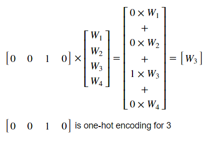
When our input vector X, which has only one 1 at the position given by input number, is multiplied with W, it essentially gives out the value at same positions from the weight matrix W. Here’s is what I mean:
Using Embeddings
In a multitude of RNN models, you’ll see embeddings beings used. Embedding are similar to one-hot encodings: An n-dimensional representation of your input(text generally) which learns the represetation along with the rest of the model.
Here, We’ll try to replace one-hot encodings with embeddings.
Input will be numbers, need to be reshaped, and before the RNN layer, there will be an embedding layer.
In :
from keras.layers import Embeddingall_feat_reshaped = all_feat.reshape(all_feat.shape[0], 3)del model
In :
input_1 = Input(shape=(3,), name='Input_Layer')
x = Embedding(input_dim=10, output_dim=10, name='Embedding_Layer')(input_1)
y = SimpleRNN(rnn_size, activation='linear', name='RNN_Layer')(x)model = Model(inputs=input_1, outputs=y)model.summary()
Out:
_________________________________________________________________
Layer (type)                 Output Shape              Param #
=================================================================
Input_Layer (InputLayer)     (None, 3)                 0
_________________________________________________________________
Embedding_Layer (Embedding)  (None, 3, 10)             100
_________________________________________________________________
RNN_Layer (SimpleRNN)        (None, 1)                 12
=================================================================
Total params: 112.0
Trainable params: 112.0
Non-trainable params: 0.0
_________________________________________________________________
In :
model.compile(optimizer=Adam(0.01), loss='mean_squared_error', metrics=['acc'])
history = model.fit(x=all_feat_reshaped, y=all_label, batch_size=8, epochs=4, validation_split=0.2, verbose=1)Train on 8000 samples, validate on 2000 samples
Epoch 1/4
8000/8000 [==============================] - 5s - loss: 4.7818 - acc: 0.7199 - val_loss: 2.5118e-08 - val_acc: 1.0000
Epoch 2/4
8000/8000 [==============================] - 4s - loss: 7.0748e-10 - acc: 1.0000 - val_loss: 8.6389e-12 - val_acc: 1.0000
Epoch 3/4
8000/8000 [==============================] - 4s - loss: 4.5370e-12 - acc: 1.0000 - val_loss: 2.4172e-12 - val_acc: 1.0000
Epoch 4/4
8000/8000 [==============================] - 5s - loss: 1.2825e-12 - acc: 1.0000 - val_loss: 9.2436e-13 - val_acc: 1.0000
Time to check predictions
In :
print('\nInput features: \n', all_feat_reshaped[-5:,:])
print('\nLabels: \n', all_label[-5:,:])
print('\nPredictions: \n', model.predict(all_feat_reshaped[-5:,:]))
Out:
Input features:
 [[0 9 3]
 [4 2 5]
 [1 5 6]
 [6 8 6]
 [6 6 6]]Labels:
 [[12]
 [11]
 [12]
 [20]
 [18]]Predictions:
 [[ 11.99999905]
 [ 11.        ]
 [ 12.        ]
 [ 20.00000191]
 [ 18.00000381]]
This time we need to check embedding weight too.
In :
embd_layer = model.get_layer('Embedding_Layer')
embd_mats = embd_layer.get_weights()wgt_layer = model.get_layer('RNN_Layer')
wgts_mats = wgt_layer.get_weights()
Embedding layer should have size = 10×10, as we’re mapping 10 numbers(integers to be precise) to 10 dimensional vectors (1 vector for each of the number). In the weight matrix, index indicates the integer to which it is mapped.
RNN weight shapes will be similar to the previous excerxise.
In:
print('Embedding W shape: ', embd_mats[0].shape)
print('W shape: ', wgts_mats[0].shape)
print('U shape: ', wgts_mats[1].shape)
print('b shape: ', wgts_mats[2].shape)Embedding W shape:  (10, 10)
W shape:  (10, 1)
U shape:  (1, 1)
b shape:  (1,)
Let’s check the weight matrices
In:
embd_matsOut:
[array([[ 0.06210777, -0.02745032,  0.03699404, -0.04357917,  0.00985156,
          0.05047535, -0.07252501, -0.0060824 ,  0.08501084,  0.02329089],
        [-0.03501924,  0.05478969, -0.06651403,  0.0606865 ,  0.07692657,
         -0.0303007 ,  0.10046678,  0.02375769, -0.00521658, -0.03262439],
        [-0.12506177,  0.09839212, -0.17181483,  0.16981345,  0.16977352,
         -0.08540933,  0.16722172,  0.15118837, -0.1214526 , -0.10981815],
        [-0.17968415,  0.25980386, -0.22894789,  0.24273922,  0.26052341,
         -0.23109256,  0.2227577 ,  0.22931208, -0.18935528, -0.25136626],
        [-0.3381401 ,  0.28742275, -0.3784467 ,  0.29970467,  0.29632148,
         -0.36220279,  0.33802927,  0.28446689, -0.31542966, -0.29835254],
        [-0.38825303,  0.43541983, -0.4055247 ,  0.43372044,  0.34076664,
         -0.40598577,  0.42293841,  0.41570613, -0.45533296, -0.40606618],
        [-0.46653211,  0.52266681, -0.48973432,  0.48285624,  0.50394773,
         -0.64239901,  0.46153784,  0.47139424, -0.55294889, -0.45976666],
        [-0.57181919,  0.57065916, -0.51719308,  0.57912141,  0.53203046,
         -0.73055142,  0.54653585,  0.59713608, -0.725555  , -0.61746806],
        [-0.69791192,  0.67029899, -0.62343609,  0.66363454,  0.69465142,
         -0.7854681 ,  0.624156  ,  0.65458065, -0.76210004, -0.65989387],
        [-0.71957815,  0.75552607, -0.76832122,  0.75740767,  0.68210703,
         -0.97855085,  0.67297399,  0.76844192, -0.93439114, -0.77425069]], dtype=float32)]
In:
wgts_matsOut:
[array([[-1.29411161],
        [ 1.12959146],
        [-1.28118789],
        [ 1.07222223],
        [ 1.29417169],
        [-0.73790312],
        [ 1.29149568],
        [ 1.28831363],
        [-0.79495221],
        [-1.01940799]], dtype=float32),
 array([[ 1.00000012]], dtype=float32),
 array([ 0.42282528], dtype=float32)]
Only U makes the sense. Remember the RNN equation:
Here, X is the embedding output. Let’s do one more transformation:
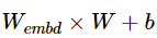
this will give us a number a vector containing 10 numbers, each corresponding to input number.
Let’s do it one by one
In :
np.matmul(embd_mats[0], wgts_mats[0])Out:
array([[-0.42282546],
       [ 0.5771746 ],
       [ 1.57717419],
       [ 2.57717466],
       [ 3.57717443],
       [ 4.57717419],
       [ 5.57717419],
       [ 6.57717371],
       [ 7.57717419],
       [ 8.57717419]], dtype=float32)
In:
np.matmul(embd_mats[0], wgts_mats[0]) + wgts_mats[2]Out:
array([[ -1.78813934e-07],
       [  9.99999881e-01],
       [  1.99999952e+00],
       [  3.00000000e+00],
       [  3.99999976e+00],
       [  4.99999952e+00],
       [  5.99999952e+00],
       [  6.99999905e+00],
       [  7.99999952e+00],
       [  8.99999905e+00]], dtype=float32)
In:
print('\n W_embd * W + b: \n', np.matmul(embd_mats[0], wgts_mats[0]) + wgts_mats[2])
print('\nU: \n', wgts_mats[1])
Out:
W_embd * W + b:
 [[ -1.78813934e-07]
 [  9.99999881e-01]
 [  1.99999952e+00]
 [  3.00000000e+00]
 [  3.99999976e+00]
 [  4.99999952e+00]
 [  5.99999952e+00]
 [  6.99999905e+00]
 [  7.99999952e+00]
 [  8.99999905e+00]]U:
 [[ 1.00000012]]
Makes some sense, right!
Let’s round it.
In :
print('\n W_embd * W + b: \n', np.round(np.matmul(embd_mats[0], wgts_mats[0]) + wgts_mats[2]))
print('\nU: \n', np.round(wgts_mats[1]))
Out:
W_embd * W + b:
 [[-0.]
 [ 1.]
 [ 2.]
 [ 3.]
 [ 4.]
 [ 5.]
 [ 6.]
 [ 7.]
 [ 8.]
 [ 9.]]U:
 [[ 1.]]
Here’s an explanation of what happened:
When you input an integer to ebmedding layer,it gives out a vector at corresponding index.
In:
embd_mats[0]Out:
array([[ 0.06210777, -0.02745032,  0.03699404, -0.04357917,  0.00985156,
         0.05047535, -0.07252501, -0.0060824 ,  0.08501084,  0.02329089],
       [-0.03501924,  0.05478969, -0.06651403,  0.0606865 ,  0.07692657,
        -0.0303007 ,  0.10046678,  0.02375769, -0.00521658, -0.03262439],
       [-0.12506177,  0.09839212, -0.17181483,  0.16981345,  0.16977352,
        -0.08540933,  0.16722172,  0.15118837, -0.1214526 , -0.10981815],
       [-0.17968415,  0.25980386, -0.22894789,  0.24273922,  0.26052341,
        -0.23109256,  0.2227577 ,  0.22931208, -0.18935528, -0.25136626],
       [-0.3381401 ,  0.28742275, -0.3784467 ,  0.29970467,  0.29632148,
        -0.36220279,  0.33802927,  0.28446689, -0.31542966, -0.29835254],
       [-0.38825303,  0.43541983, -0.4055247 ,  0.43372044,  0.34076664,
        -0.40598577,  0.42293841,  0.41570613, -0.45533296, -0.40606618],
       [-0.46653211,  0.52266681, -0.48973432,  0.48285624,  0.50394773,
        -0.64239901,  0.46153784,  0.47139424, -0.55294889, -0.45976666],
       [-0.57181919,  0.57065916, -0.51719308,  0.57912141,  0.53203046,
        -0.73055142,  0.54653585,  0.59713608, -0.725555  , -0.61746806],
       [-0.69791192,  0.67029899, -0.62343609,  0.66363454,  0.69465142,
        -0.7854681 ,  0.624156  ,  0.65458065, -0.76210004, -0.65989387],
       [-0.71957815,  0.75552607, -0.76832122,  0.75740767,  0.68210703,
        -0.97855085,  0.67297399,  0.76844192, -0.93439114, -0.77425069]], dtype=float32)
In :
# If input was '5', output will be
embd_mats[0][5]
Out:
array([-0.38825303,  0.43541983, -0.4055247 ,  0.43372044,  0.34076664,
       -0.40598577,  0.42293841,  0.41570613, -0.45533296, -0.40606618], dtype=float32)
This input is similar to one-hot encoding.
In the next step(RNN), this vector get multipled to W to produce a vector of rnn_size, which in this case is 1, so it gives out one number in our case.
As you could see, embeddings learn represetation in combination to other matrices and thus might be difficult to explain directly.
Here’s the link to corresponding notebook. The steps will look much cleaner there.